Which songs received the most points?

Starting off simple, let’s take a look at the songs that received the most points. Each of the 300+ songs received at least 2 points, so we’ll limit the plot to the top ten.

# Top 10 songs 
artist_rankings %>% 
  top_n(10, points) %>% 
  mutate(title_artist = paste0(title, "\nby ", artist),
         title_artist = fct_reorder(title_artist, points)) %>% 
  ggplot(aes(x = title_artist, y = points)) + 
  geom_col(fill = "steelblue") + 
  coord_flip() + 
  theme_minimal() + 
  theme(axis.text.y = element_text(hjust = 0)) +
  labs(title = "Which songs received the most points?",
       x = "",
       y = "Total points")

What is the distribution of nominated song releases and song points over time?

Hip-hop has a very interesting history and the next thing that I wanted to look at was the how the release years and total points of these 300+ nominated songs were distributed over time.

# Number of nominated songs released per year
artist_rankings %>% 
  count(year) %>% 
  ggplot(aes(x = year, y = n)) + 
  geom_col(fill = "steelblue") + 
  theme_minimal() + 
  labs(title = "Number of nominated songs released per year",
       x = "Year",
       y = "Number of songs")

# Total number of points awarded per year
artist_rankings %>% 
  group_by(year) %>% 
  summarize(yearly_points = sum(points)) %>% 
  ggplot(aes(x = year, y = yearly_points)) + 
  geom_col(fill = "steelblue") + 
  theme_minimal() + 
  labs(title = "Number of song points awarded by release year",
       x = "Year",
       y = "Points")

Both plots show a significant increase in the 90s, which is consistent with the genre becoming a best-selling music genre in the mid-1990s and the top selling music genre by 1999.

What is the distribution of artist genders?

The next thing I wanted to look at was the gender distribution of artists in the list of nominated songs.

# Artist gender distribution
artist_rankings %>% 
  count(gender)

## # A tibble: 3 x 2
##   gender     n
##   <chr>  <int>
## 1 female    23
## 2 male     267
## 3 mixed     20

With 267 of the 300+ nominated songs having male artists, we can definitely notice how male-dominated the space is.

It is important to note that the numbers above are counting duplicates of artists who produced multiple songs in the list of 300+ nominated songs.

For unique artists, we can do this:

# Artist gender distribution, no duplicates
artist_rankings %>% 
  distinct(artist, .keep_all = TRUE) %>% 
  count(gender)

## # A tibble: 3 x 2
##   gender     n
##   <chr>  <int>
## 1 female    18
## 2 male     169
## 3 mixed     20

However this still doesn’t account for artists collaborating with different combinations of other artists. We could extract artists featured in songs (by extracting names separated by “ft.”, “feat”, “and”, and “&”), but not all are hip-hop artists and it would require additional work to determine the gender of the artists from gender-mixed collaborative songs.

# Distribution of artist genders over time
artist_rankings %>% 
  group_by(year, gender) %>% 
  count(gender) %>% 
  ggplot(aes(x = year, y = n, fill = gender)) +
  geom_col() + 
  facet_wrap(~gender) +
  theme(legend.position = "none") +
  labs(title = "Number of songs per artist gender over time",
       x = "Year",
       y = "Number of songs")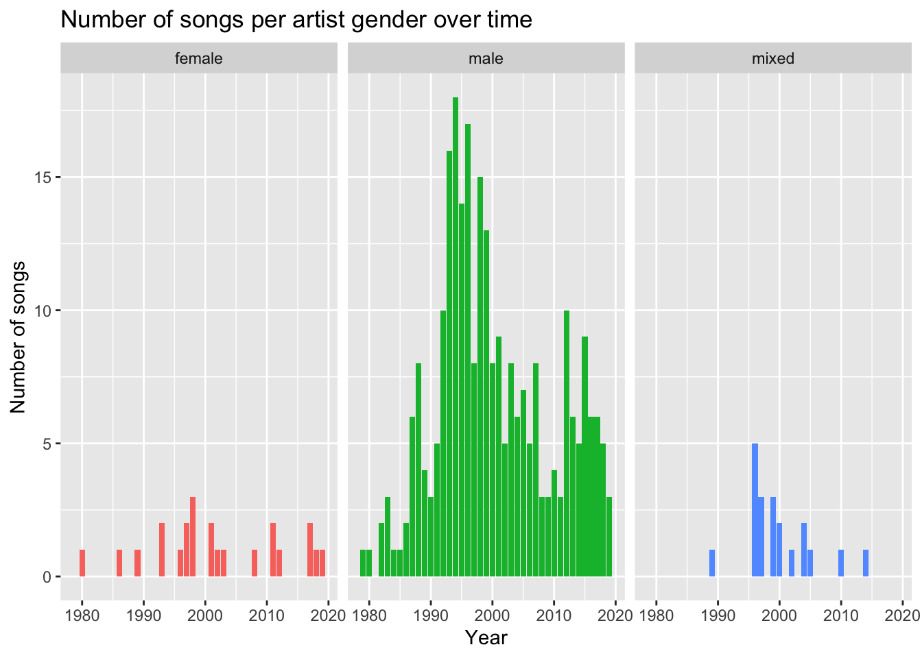

Visualizing points, gender, and time together

Now that we’ve taken a look at points, gender, and time separately, let’s view how they all interact together.

# Points over time by gender
artist_rankings %>% 
  ggplot(aes(x = year, y = points, color = gender, label = title)) +
  geom_jitter(alpha = 0.6) + 
  geom_text(aes(label = ifelse(points >= 50, title, "")), 
            color = "black", 
            hjust = -0.1, 
            vjust = 0) +
  scale_color_brewer(palette="Set1") +
  theme_minimal() +
  labs(title = "",
       x = "Year",
       y = "Total points",
       color = "")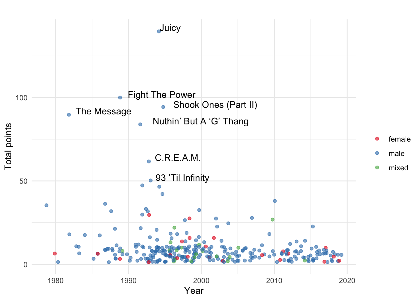

What is the distribution of critics’ roles?

While the votes/points for these songs were done by critics, industry figures, artists, academics in the field of hip-hop and music, it is important to keep in mind that music is a subjective field. We can take a quick look at some of the top roles of those critics:

# Top critic roles
artist_polls %>% 
  distinct(critic_name, .keep_all = TRUE) %>% 
  mutate(role_lump = fct_lump(critic_rols, 6)) %>% 
  count(role_lump, sort = TRUE) %>% 
  mutate(role_lump = fct_reorder(role_lump, n)) %>% 
  ggplot(aes(x = role_lump, y = n)) +
  geom_col(fill = "steelblue") + 
  coord_flip() + 
  theme_minimal() + 
  labs(title = "What is the distribution of critics' roles?",
       x = "Critic's role",
       y = "Number of critics")

While there does exist a large range of unique companies and roles, the label “Critic” is the only consistently specific role, which isn’t quite descriptive enough to draw further insight from. The rest of the roles in “Other” are unique enough (each only existing once) that they are not able to be generalized further without manual classification.

What is the distribution of critics’ primary country?

The last thing I wanted to investigate was the countries from which the critics were taken from.

# Plot critic primary countries
artist_polls %>% 
  distinct(critic_name, .keep_all = TRUE) %>% 
  count(critic_country) %>% 
  mutate(critic_country = reorder(critic_country, n)) %>% 
  ggplot(aes(x = critic_country, y = n)) +
  geom_col(fill = "steelblue") + 
  coord_flip() + 
  theme_minimal() + 
  labs(title = "What is the distribution of critics' primary country?",
       x = "Critic's country",
       y = "Number of critics")

Given the fact that hip-hop originated and developed in the United States, it is not surprising that the majority of the critics polled were from there. This does give a bit more context to the statement “We polled 108 critics from 15 countries across six continents” by the BBC. It is interesting to see critics from countries that I hadn’t expected, such as China, Japan, India, and Russia.

Check out the code for this project on GitHub!